Applying a size standard template

Applying a Size Standard Template

Previous Top Next

Size standard

A size standard is a mixture of DNA fragments with known fragment lengths. It is used to calibrate the fragments of samples where the fragment lengths are unknown.

Prerequisites for the calibration process

The size standard calibration process requires the following information:

1. the peak locations in the size standard channel/lane (a peak detection prior to the calibration process) and

2. knowledge of the base sizes of each fragment.

Although each electrophoresis run is unique it would be very time consuming to assign the bands in the size standard lane for each run manually. Therefore, a size standard template is defined and can be applied to any sample containing this size standard.

Size standard templates

A size standard template contains the mobility and the base size for each peak of an exemplary electrophoresis run. Of course, a 'good' run will be used to define a size standard template.

Table 1 shows how a size standard template for the 'ABI GeneScan 50-500' size standard could look like. This size standard contains 16 fragments. The fragment with a length of 248 bases often runs atypically and, therefore, is usually not included into the size standard template.

Size standard calibration process

The size standard calibration process applies a size standard template to the detected peaks in a size standard lane of a sample. In fact the mobility data of both data sets are compared and the best path using some kind of error function is found. Then the base sizes are assigned to the peaks in the sample.

The task is to assign the right base size labels to these peaks using the values of Tab.1.

Figs. 2 and 3 show two trace curves before and after applying a size standard template.

Tab. 1. Peak data of a size standard template (ABI GeneScan 35-500). Each row contains a data point value (the midpoint of a peak) and its corresponding base size.

Data point	Base Size
2186	35
2460	50
2915	75
3340	100
4001	139
4173	150
4341	160
5012	200
6649	300
7269	340
7435	350
8213	400
8947	450
9521	490
9651	500

Tab. 2. Data point values of peaks as detected in the size standard channel of a sample run.

Data point
62
789
1452
2490
2512
2764
2788
3055
4142
4172
5481
5510
6984
7013
8109
8134
8440
8467
9951
9981
11424
12540
12794

Fig. 1

Comparison between the peak mobilities in the size standard channel of a sample and the pre-defined mobilities of a size standard template. The values were taken from Tab. 1. (ABI GeneScan 35-500 size standard). The green dots indicate the optimal path through the two data sets.

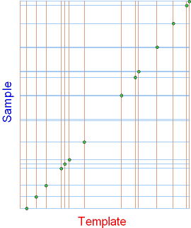
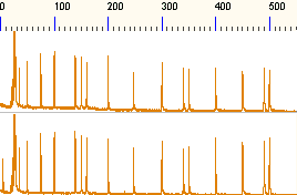
Fig. 2. This image shows two sample runs with the same size standard.

The data is scaled by data points, i.e. according to the temporal appearance. In the second sample, the sample peaks appear earlier and in a shorter time interval. The whole sample appears 'compressed' if compared with the first one.

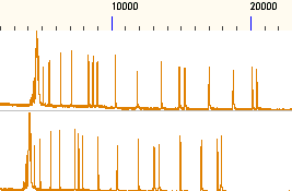
Fig. 3. The same data as in Fig. 2 but after a calibration using a size standard.

Each peak obtained a base size label and the samples can now be scaled by base sizes, i.e. the real fragment lengths.

See also

> Sizing